Financial cycles
Disclaimer: This post (like all others) represents my opinion alone and should not be attributed to De Nederlandsche Bank, the Eurosystem or, indeed, anyone else.
tl;dr Financial cycles, the way they are commonly defined, do not exist separately from the business cycle. Evidence for separate credit cycles is artificially constructed via a stock-flow mismatch.
An increasing number of papers are appearing on the topic of financial cycles, including the papers presented at a DNB workshop I attended recently. In the papers of this workshop, financial cycles were defined as cycles in outstanding credit to the non-financial sector. The assumption is that credit cycles are distinct from business cycle as defined via GDP and that these different cycles are interesting to understand from a policy point of view.
As an example of what this might look like consider the graph below that plots consumption and investment (C+I) growth together with credit growth for the US. I use consumption and investment growth as the credit plotted in the graph (and used in the papers of the workshop) is to the private, non-financial sector only.
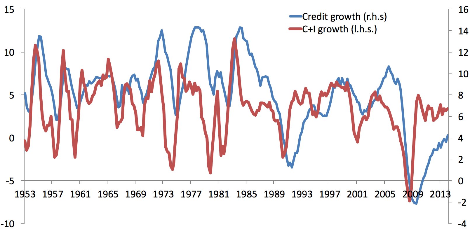
Notice that in the early and late 1970s and the mid 1980s credit growth does not seem to be synchronized with C+I growth. The most recent event where this divergence appeared was the recovery from the financial crisis in 2009. C+I growth recovers relatively swiftly but credit growth has the trough only a few quarters later. This led Calvo and Loo-Kung to call the US recovery a “Phoenix miracle” in a VOX EU column.
However, there is a major problem with the graph above: consumption and investment are flow variables and credit is a stock variable; comparing them is a stock-flow mismatch. This means that in the above graph the expenditures in a given period are compared to the credit that firms and households have taken out in the past (and not repaid yet). However, it is fairly intuitive that expenditures in a given period are most closely related to borrowing of that period. Together with Mike Biggs and Thomas Mayer, I discussed this problem in the context of credit-less recoveries (Biggs et al., 2010); a more concise explanation of the issue is available in our VOX EU column.
In place of the stock of credit, compare C+I to the flow of credit, that is, to the net new borrowing in each period (below I write how we approximate this). In the graph below are C+I growth and the growth of the flow of credit, which Biggs et al. (2010) call the credit impulse.
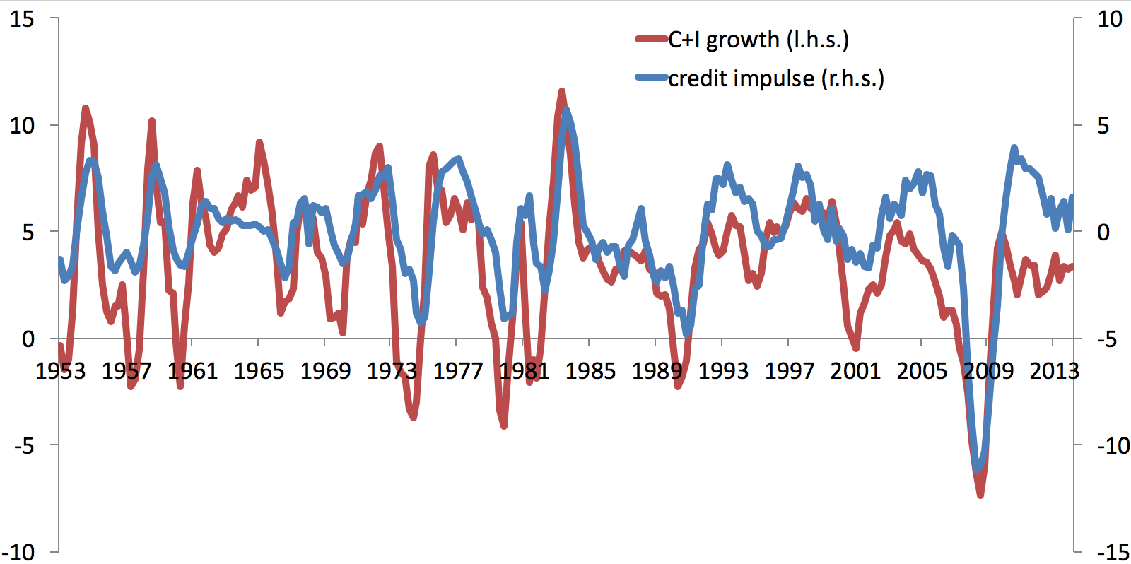
It is clear that all the anomalies that appeared in the previous graph are now gone. The recovery from the financial crisis in 2009 are equally fast for C+I as for the flow of credit.
An important insight from the credit impulse is that economies can recover while they are deleveraging. The logic is simple: Assume your income is fixed at 100, and that you have to repay 10 units of currency in one period and 5 units in the next. In both periods, you are deleveraging but your consumption in the second period will be 5 units larger than in the first: consumption growth will be positive. This occurs while credit is still shrinking (you are repaying 5) but the flow of credit has increased from -10 to -5.
How, then, did so many economist fall for a stock-flow mismatch?
My best guess, based on the presentations in the workshop, is the following. Assume that firms borrow to invest, pay interest r on existing credit, and investment is a fixed proportion of GDP. Then
(1) C(t) = (1+r) C(t-1) + I = (1+r) C(t-1) + g*Y
where C is the stock of credit, I is investment, Y is GDP, r is the interest rate, g is a constant, and t denotes discrete time. (And despite the notation, this is in discrete time – clearly, I need to get mathjax up and running.)
There is an equilibrium relationship between GDP and credit, which is
(2) C = b*Y
where b is a constant that is comprised of the deeper parameters of the economy. Hence, in equilibrium, the stock of credit and the flow of GDP are related. Drehmann and Juselius (2016, Bank of Finland WP) derive a similar equilibrium relationship (in a more elaborate model). They then assume that this equilibrium holds at all times except for a disturbance term.
However, it is clear that
(3) C(t) = b*Y(t) + e(t)
behaves fundamentally different from the dynamics in equation (1) from which the equilibrium was derived. As Brainard and Tobin (1968, AER, p.105) wrote:
“No one seriously believes that either the economy as a whole or its financial subsector is continuously in an equilibrium. Equations like those of the model described above do not hold every moment in time. […] There are, of course, identities–e.g. balance sheet or income identities–that apply out of equilibrium as well.”
For the description of financial crises and recoveries it should be clear that the equilibrium is not a good description of the economy but that the credit identity will hold in each period. Rewriting equation (1) yields
(4) C(t) - (1-r) C(t-1) = g*Y
that is, domestic, private demand is related to the net flow of credit. A complication is that the interest rates that are used for private credit is generally not observed. It could be approximated by a 10 year corporate bond rate or a similar interest rate. In the graph above, I approximated the net flow by the difference of credit as I found in previous work that this yields a reasonably good approximation as long as interest rates are not too high.
In conclusion, I hope that it has become clear that credit cycles that are distinct from the business cycle do not exist, that they should not be artificially constructed via stock-flow mismatches, and that analyzing stock-flow mismatch relations cannot lead to valid insights.